In periodogram analysis of data with measurement errors, one must make a critical decision about where to draw the line between what is interpreted as a real signal and what could be just a signature of noise. Typically I am analyzing time series measurements of brightnesses of stars with the Fourier transform or the Lomb-Scargle periodogram, and I want to know if the star is varying significantly in brightness, or if the measurements are consistent with what we expect for noisy measurements of a constant-brightness source. My approach is to consider whether any peaks in the periodogram are tall enough to be exceedingly unlikely to represent noise. A periodogram peak must be as tall as the “significance threshold” for me to believe it represents a real signal.

I go over some of the basics of periodogram analysis in my previous post “How data sampling affects the Fourier transform periodogram.” The animated periodograms in that post include a line at 4 times the average amplitude in the periodogram as an approximate significance threshold, but careful data analysis should adopt a threshold level that is deliberately chosen to be appropriate for the problem at hand. This post will demonstrate how to calculate a statistical threshold with bootstrap resampling.

Consider the periodogram below of a pulsating white dwarf star observed by NASA’s TESS satellite under the target name TIC 188087204.

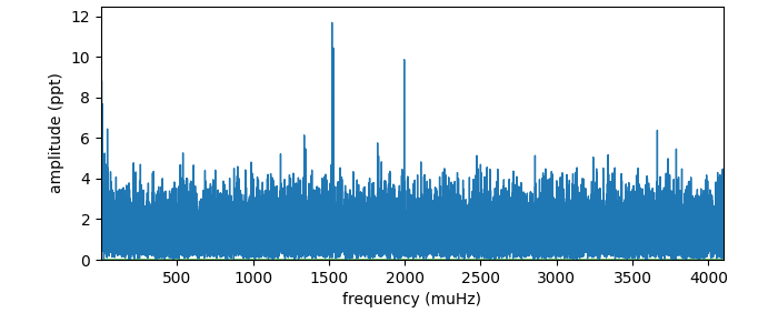
This is the amplitude spectrum (square root of the power spectrum on the y axis, in units of parts-per-thousand), showing what the best-fit amplitude is for a series of sinusoids with different frequencies (sampled on the x axis in units of microHertz from zero to the Nyquist frequency). This is the frequency-domain representation of 60 days of brightness measurements of a white dwarf star taken every 2 minutes, with considerable measurement noise affecting each data point. The noise manifests in the periodogram as a noise floor of peaks with a range of heights distributed across all sampled frequencies. This might look like the grass of an unkempt lawn growing along the bottom of the plot. It is apparent in the periodogram shown above that some peaks stick out taller than others. The question of significance, in the lawn analogy, is whether the tallest peaks are dandelions (signal) or just the tallest of the many blades of grass (noise).

Here is a histogram of amplitude values sampled by the periodogram above (counts shown on a logarithmic scale).

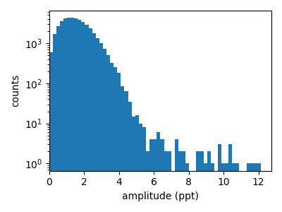
The low-amplitude end of the distribution is well sampled with upwards of thousands of samples per bin, while the high-amplitude tail of the distribution is poorly sampled. More confusing yet, this periodogram was “oversampled,” meaning that the frequencies were sampled more densely than the frequency resolution so there is more than one point for each peak of the periodogram, and these samples are not independent.

Under some idealized assumptions (even time sampling with uncorrelated Gaussian-random error), the noise amplitudes would follow a known distribution that we could use to estimate a significance threshold (Chi with 2 degrees of freedom described more here and here). Real data violate these assumptions, so we estimate the threshold empirically instead.

Acknowledging the risk that we might misinterpret a tall noise peak as genuine signal, we must adopt some risk tolerance. Since we might understand the distribution of peaks due to noise, we can calculate an amplitude threshold above which only in exceptionally (but acceptably) rare circumstances would noise conspire to produce such a peak. This threshold is typically set to correspond to a calculated false alarm probability (FAP). The FAP is the probability that a random data set like yours could produce a noise peak that would exceed the threshold. Perhaps a 1/1000 risk would be tolerable for your data analysis, as a reasonable trade-off between risking a false detection and potentially missing a real signal. For an analytical distribution like a 2-degrees-of-freedom Chi distribution, this threshold can be set at the location where the cumulative density function (integrated probability density function) equals 1 - FAP, e.g, 0.999 for FAP = 1/1000.

Unfortunately, real data sets generally don’t satisfy the assumptions that would exactly produce precisely Chi-distributed amplitude noise: the time sampling may not be evenly spaced, and the errors may be non-Gaussian or vary with time. Your results are so sensitive to where you set the significance threshold that the choice should be carefully considered.

One approach to calculating a threshold based on the properties of your actual data is bootstrapping. Here we assume the “null hypothesis” that the time series contains only noise of unknown distribution, and then we will test whether we can reject this hypothesis and recognize a significant peak in our data set. We still assume that the errors are uncorrelated and consistent across the observations, but the distribution is unknown. Since we don’t know the analytic noise distribution, we treat the distribution of observed fluxes as an empirical proxy for the noise distribution under the null hypothesis. If each measurement in the time series is just one realization of the noise distribution, then under the null hypothesis we assume the noise distribution looks like this histogram:

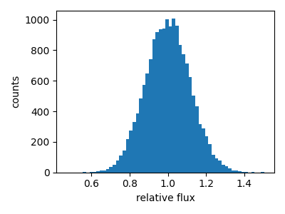
We can then use this empirical distribution to draw random noise time series to see how high of a peak in the periodogram we can reasonably expect noise to produce on its own. To do this, we want to draw from this distribution (with replacement, since the noise is independent) new values of noise to assign to each time series observation in our data set. By keeping the same timestamps of the original data, the resulting periodogram will be based on the actual sampling and observed noise behavior of the data.

This function resamples time series light curve values from the original light curve (stored as a lightkurve.LightCurve object).

def bootstrap(lc):
    # redraw flux with replacement from the provided light curve
    bootstrappedlc = lc.copy().remove_nans() # Make a copy and remove nans
    N = len(bootstrappedlc) # Number of samples to draw
    rng = np.random.default_rng() # Random generator thingie
    bootstrappedlc.flux = rng.choice(lc.flux.value,N,replace=True)*lc.flux.unit # Replace flux
    return bootstrappedlc.normalize() # Normalize before return

It is important to include any preprocessing steps that you would apply to your actual data before computing the periodogram, like normalizing the light curve to have an average value of 1. By randomizing the data set, we surely destroy any correlations caused by signals that may be present, and any intrinsic variability is swept into the treatment of noise for the moment.

If we compute periodograms from many of these bootstrapped time series, assuming still that all values in the time series represent the effect of noise, we can observe how high a noise peak can rise in the periodograms. The periodogram should be computed identically to the periodogram of your original data. If we want to know the amplitude threshold above which there is only a false alarm probability (FAP) of 1/1000, we should simulate thousands of bootstrapped periodograms and record the 99.9th percentile of highest peak found in each periodogram.

Here is the histogram of the highest amplitude peak found in periodograms of each of 10,000 randomized data sets under the null hypothesis.

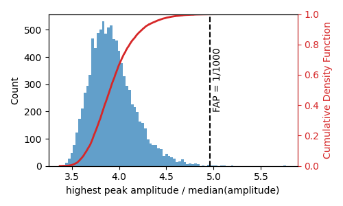
The amplitudes are recorded relative to the median amplitude across the periodogram, and we find for this data set that it is quite common for the highest peak due to noise to rise above 4 times the median amplitude. The red curve shows the cumulative density function (CDF) that integrates to one across the histogram. The FAP = 1/1000 is recorded where the CDF = 0.999, as marked with the vertical dashed line. While we could estimate this value from 1000 random data sets, it would be a noisy estimate determined mostly by the single most extreme value in the tail of the noise distribution. In this example, the 1/1000 FAP level is estimated at 4.96 times the median, while the single most extreme amplitude value reached 5.77 times the median (a noisy estimate of the 1/10000 FAP level).

We often record the peak amplitude relative to the median because in the real data, there can be some correlated noise that causes the local noise level to change gradually across the periodogram. The significance threshold determined from bootstrapping is then often applied locally in the periodogram relative to the median amplitude computed across a local frequency range. For our white dwarf light curve, here is the periodogram again with the FAP = 1/1000 threshold marked at 4.96 times the median.

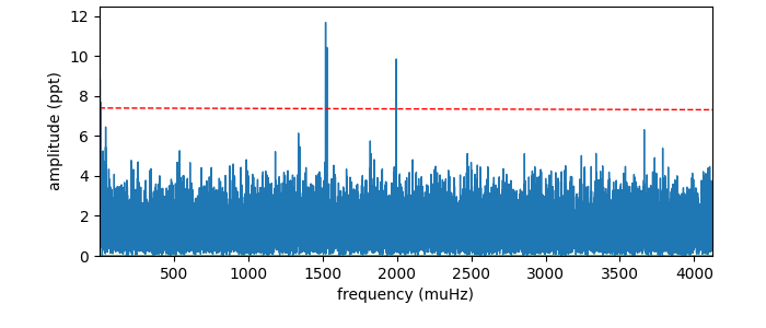
The peaks near 1500 and 2000 microHz rise well above this significance threshold. Under this noise-only bootstrap model, peaks this high would occur in fewer than about 1 in 1000 trials. This allows us to reject the null hypothesis that the data contain only noise. We believe that these represent real signals and can interpret them as such. The presence of these signals will have inflated the distribution of noise we used for testing the null hypothesis. Since we do not believe these peaks represent noise, we could fit and remove these signals from the time series and repeat the bootstrapping procedure on the residuals to test if there are any additional signals. This is a typical part of the pre-whitening procedure for periodogram analysis that I am writing a more formal tutorial paper about.