You’re likely familiar with the 68–95–99.7 rule that gives the percentage of a Gaussian distribution contained within 1-2-3 standard deviations. It’s more of a mnemonic for remembering these useful values, which are often used in rule-of-thumb significance estimation. Gaussians come up all the time in practice, often as approximations to probability distributions. In significance testing, one often wants to know how likely it is for some random value to have been drawn at its distance out into the exponential tail of a Gaussian distribution. This characteristic of a distribution is referred to as the “confidence interval” or the “credible interval,” depending on philosophy. See this post from Jake VanderPlas for a discussion of the different interpretations. I won’t be particularly careful about my language here.

But I’m interested in 2D distributions at the moment (though these ideas should extend higher), and distributions that may not be Gaussian. For these I want to compute confidence/credible regions. Specifically, for some point drawn from a probability density distribution (pdf), I want to know what percentage of other random values would be drawn from higher-likelihood locations. Mathematically, this is the integrated volume under the region of a (normalized!) pdf that exceeds the value at the selected point.

For this problem, I will use a Gaussian mixture model (GMM), though the approach should work for any normalized pdf. In fact, GMMs are often used to fit more complicated pdfs. They also come up in classification/clustering algorithms. I’ll use scikit learn’s GMM class for this tutorial (their documentation on GMMs is great), though I really like the advanced fitting capabilities of the pygmmis package.

We use this sklearn demo script as a launching off point. The one modification is to sample the x and y dimensions with in steps of 1 by swapping np.arange for np.linspace.

x = np.arange(-20.0, 30.0)
y = np.arange(-20.0, 40.0)

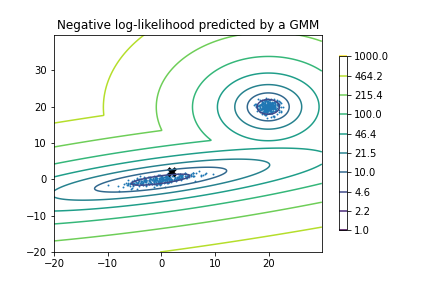
A 2-component GMM is fit to simulated data, stored as the mixture.GaussianMixture object clf. A contour plot is also made to indicate the shape of the distribution. The pdf is a density function in the units of its parameters, so a nice consequence of sampling in steps of one is that we can integrate the pdf over the sampled space by summing the values

np.sum(np.exp(-Z))

which gives 1.0000000317591327, a reasonable value for the probability of something happening somewhere given limited numerical precision. Sampling the space in steps of l, the probability can be integrated as np.sum(np.exp(-Z))*l**2.

A concern comes to mind: what is a sufficient sampling step to for a reliable numerical integration? If we sample with steps that are too large, we may miss (or mischaracterize) narrow features of the pdf. Making sure that we integrate over a sufficiently large area to capture the regions of significant probability is a similar concern. To be sure these decisions are made appropriately, I integrated a single 2D Gaussian with different step sizes and boundaries. The results are shown below, where step sizes and boundary half-widths are given relative to the Gaussian scale parameter, sigma.

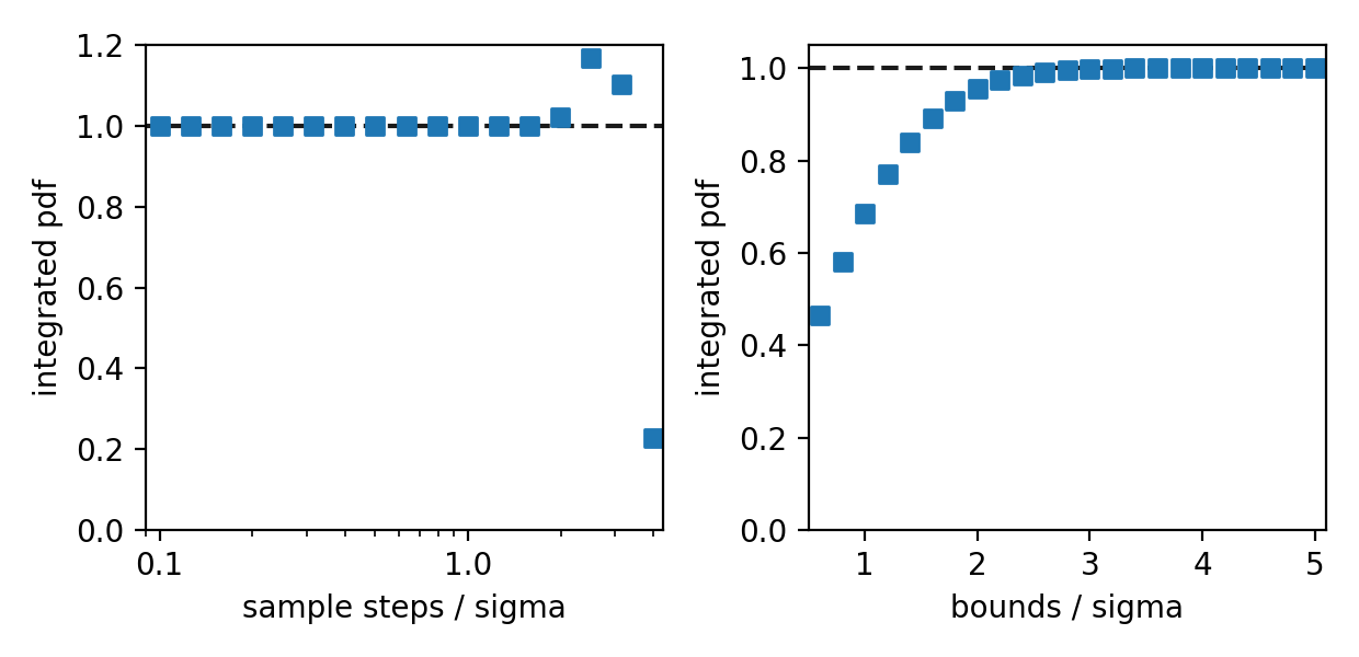
At large step sizes and small integration bounds, the total integrated probability diverges from 1.0 as we’d expect. Inspecting more closely, we appear to achieve results good to one part-per-million for all step sizes smaller than sigma, and for integrations that contain the inner 5-sigma regions. For a GMM we should ensure that our sample steps are smaller than the scale parameter of the narrowest Gaussian, and that we sufficiently encompass all components. A way to check that a sufficient area of the pdf has been sampled using contours is given at the end of this post.

Back to the GMM from the scipy example. Say we measure a single event occurring at position (2,2) that we think may have been generated from this GMM pdf. This point is marked with an X on the contour plot below. Is this value consistent with being drawn from this distribution with some reasonable probability? Certainly there are locations where it would have been more likely to randomly observe this event. The question we want to answer in computing credible regions is: what is the probability that we would have observed such an unlikely event from this distribution?

We can evaluate the pdf at the (2,2) location to obtain the (natural) log likelihood denisty of an event occurring here:

lnL = clf.score_samples([[2,2]])

equal to -6.6755, or L = 0.0012615.

Finally we can get the probability that the data would have been drawn from a more likely location by numerically integrating the pdf where sampled lnL is greater than at the observed point, and subtracting this from 1.0:

p = 1 - np.sum(np.exp(-Z[-Z > lnL]))*stepsize**2

which gives effectively a p-value of 0.0256. In English, we’d only expect such an unlikely value to be drawn from this distribution in 2.56% of realizations. Whether you consider this probability to be comfortably consistent with the overall distribution will depend on the problem at hand.

Here’s the same plot with a contour drawn through the point (2,2) by setting the contour level to the corresponding lnL value.

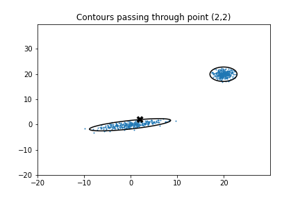
It looks like about 2.5% of the sampled points do, in fact, fall outside of these contours as we now expect. It’s good that these contours appear completely closed, as this means that we didn’t miss any probability density when we summed over the higher values. This statement makes the important assumptions that we sample the distribution finely enough to resolve local extrema and that all local maxima are contained within the sampled area.

That leads to a way to check that the pdf is sampled far enough out into the wings for a reliable numerical integration using contours. I use find_contours of the scikit-image package to compute contours at a given log likelihood level. A closed contour will end and start at the same point. A contour that leaves the sampled footprint will not. For a GMM, there may be multiple contours at a given level, and they should all be closed. Here’s how I check:

from skimage import measure

# Compute contour at point (2,2)
contours = measure.find_contours(Z, -clf.score_samples([[2,2]]))

def pathclosed(contour):
    # Does this contour end where it starts?
    return np.all(contour[0] == contour[-1])
def allclosed(contours):
    # Are all contours closed?
    return np.all([pathclosed(contour) for contour in contours])

allclosed(contours) #True

The function reports that the contours that pass through the point (2,2) are closed in the footprint (sampled from -20 to 30 in X, -20 to 40 in Y). On the other hand, the contour that passes through point (0,10), for example, is not closed and the integrated probability over the sampled area would be underreported.

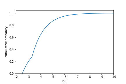
Finally, we might want to know the pdf value (or draw contours) corresponding to a specific p-value. For this, we sort the sampled lnL values from largest to smallest, then map that to the cumulative sum. This gives the amount of integrated probability down to a given pdf value, which we can then interpolate to a probability level of interest.

from scipy.interpolate import interp1d

sortlnL = np.sort(-Z.flatten())[::-1]
cumsum = np.cumsum(np.exp(sortlnL)*stepsize**2)

# Make interpolator
lnLatpvalue = interp1d(1-cumsum,sortlnL)

# Evaluate at p-value of interest
pvalue = 0.05
lnLatpvalue(pvalue)

This cumulative distribution gives the integrated probability over areas more probable than a given lnL value. For this example, 95% of distribution is contained within an lnL value of around -6.

The Jupyter Notebook I used for this analysis is available at here.