I find myself working out the relationship between the noise in time series data to the noise in the periodogram represented as an amplitude spectrum (Fourier transform) occasionally, so I’m writing it down somewhere I won’t lose it. I agree with the statement from “Asteroseismic Data Analysis: Foundations and Techniques” by Sarbani Basu and Bill Chaplin (Section 5.1.4)

Belt-and-braces checks of the [power spectrum] calibrations may be made by considering limiting dataset cases comprising of either white noise or commensurate sinusoids. It is extremely useful to be able to make a quick back-of-the-envelope prediction of the expected power spectral density for the white-noise case. This provides an estimate of the shot noise background we would expect given known photon-counting rates.

They go on to show that for the power spectrum, calibrated via Parseval’s theorem (total power in time series = total power in power spectrum), the average power per frequency bin is \(2\sigma^2/N\), where \(\sigma\) is the relative flux uncertainty (assumed stationary), and \(N\) is the number of time series points. This is a nice result for the power spectrum, where white noise will be distributed about this level as \(\chi^2\) with two degrees of freedom. This distribution has some convenient properties that make it relatively easy to work with, as demonstrated in my post “Fitting features in a power spectrum with least squares and MLE.”

However, in many studies of time series variability, the amplitude spectrum is preferred to the power spectrum, and is simply the square-root of the power spectrum (depending on normalization convention, but at least proportional). I prefer the amplitude spectrum when I am fitting models in the time domain rather than the frequency domain. The height of a peak in the amplitude spectrum can tell you directly the amplitude and frequency of a best-fit sinusoid in that frequency bin. The highest points in the power spectrum (squared amplitude spectrum) will appear to stick out above the noise more dramatically to the eye, so my colleague Michel Breger taught me another, perhaps psychological reason to prefer working with the amplitude spectrum: you’ll be less likely to convince yourself that a noise peak is signal when looking at the amplitude spectrum. I haven’t generally taken the other side of his advice (given at least part jokingly): plot the power spectrum in publications to convince readers that the signals you claim to have detected are real!

Despite how much I want it to be true, the average value of the white noise amplitude spectrum is not the square-root of the average noise in the power spectrum. The square root is not a linear operator, and therefore the shape of the noise distribution changes… for the worse. While the noise distributed as \(\chi^2\) with 2 degrees of freedom in the power spectrum has a straightforward value for the mean, the noise in the amplitude spectrum is distributed as a Chi distribution with 2 d.o.f., where the mean value involves a dreaded gamma function evaluation. Long story short, we have to multiply the square-root of the average noise in the power spectrum, \(\sigma\sqrt{2/N}\), by the ratio of the mean to the scale parameter for a \(\chi\), 2 d.o.f. distribution. We can get this coefficient easily with SciPy.

from scipy.stats import chi
print(chi.stats(df=2, loc=0, scale=1, moments='m'))

1.2533141373155003

i.e., \(\sqrt{2}\Gamma(3/2)\).

And as always, check this with some simple simulations, here using the Lightkurve package.

import lightkurve as lk
import numpy as np

#Generate white noise light curve
sigma = 0.02 #Gaussian flux error
N = 10000 #Number of time series samples
lc = lk.LightCurve(time=np.arange(N), flux=1 + sigma*np.random.randn(N))

#Compute amplitude spectrum
per = lc.to_periodogram(normalization='amplitude')
meanamp = np.mean(per.power.value) #power is a misnomer

c = chi.stats(df=2, loc=0, scale=1, moments='m')
expectedmean = c*sigma*np.sqrt(2/N)

print(expectedmean, meanamp)

0.00035449077018110325 0.0003565418892748973

Close enough for me. That’s the difference between the expectation value for the mean, and the actual mean for this realization of noise. Unfortunately the usual notation for expectation value is often used in the literature to refer to the measured average amplitude: \(\langle A\rangle\). Here’s results of a bunch of noise realizations that show that the average average amplitude converges to the expectation value, as expected.

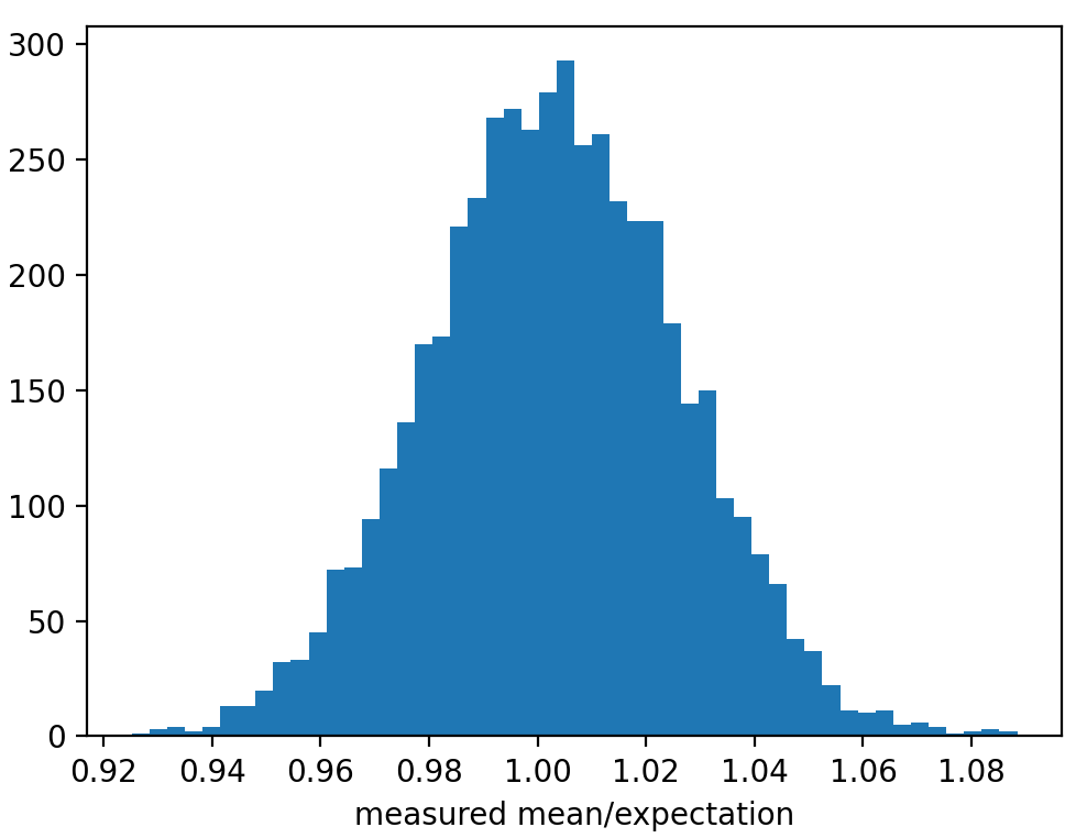
The point: the expectation value for the mean of the Fourier amplitude spectrum of a Gaussian white noise time series with standard deviation \(\sigma\) and \(N\) points is \(\langle\bar{A}\rangle = 1.2533141373155 * \sigma\sqrt{2/N}\); or, if you prefer gamma functions to ugly coefficients: \(\langle\bar{A}\rangle = 2\sigma\Gamma(3/2)\sqrt{1/N}\).