This is a stupid way to fit a sinusoid to data.

I was recently discussing with a colleague how to determine the relative probabilities that a few different test parameters for our model describe some data. Since we have only a few discrete combinations of values to test, I suggested that we could just test every combination and use the the likelihood function to convert the \(\chi^2\) goodness-of-fit statistic into probabilities. My description of how I’ve seen this done for searches of asteroseismic model grids was met with some skepticism, but my colleague said he might believe me if I could reproduce a classic result like fitting a sinusoid to data. For a signal with known frequency, could I recover the amplitude and phase input to noisy simulated data, as well as uncertainties that agree with analytical expectations for least-squares fitting? It sure sounds silly (and inefficient) to fit a sinusoid with a grid search over a range of values for the amplitude and phase parameters, but a good proof-of-concept!

Here’s the setup:

# Define the sinusoid to be recovered
freq = 0.001   	#assume known
amp = 0.06     	#find with grid search
phase = 0.7    	#find with grid search

# Sample this sinusoid at a series of times
tsample = np.arange(0,8*3600,60) #8 hours observations every minute

# Underlying sinusoidal signal
signal = amp*np.sin(2.*np.pi*(freq*tsample + phase))

# Add Gaussian noise
noise = 0.1  	#stddev greater than sin amplitude
measures = signal + noise * np.random.randn(tsample.size)

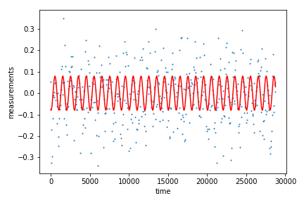
# Plot the data
plt.scatter(tsample,measures,s=1)
plt.plot(tsample,signal,c='r')
plt.xlabel('time')
plt.ylabel('measurements')
plt.tight_layout()
plt.show()

I am going to fit a single sinusoidal model to this time series, which could be easily done with least squares or direct maximum likelihood estimation. But we could have a much more complicated model, where each model computation takes hours or days. It would be expensive to compute these on the fly as we fit the data. Instead we might pre-compute a grid of models, sampling different values for the model parameters. Let’s do this for the sine model just to show how it works, sampling phase and amplitude spanning the values underlying the simulated data.

# Sample phase and amplitude
phasesample = np.linspace(0,1,201)
ampsample = np.linspace(0.001,0.1,201)
# Create grid of all amplitude, phase combinations to be tested
ampgrid,phasegrid = np.meshgrid(ampsample,phasesample)

And let’s define the model that we will compare to the data. We assume here that the underlying frequency is known. Note that an important assumption of this process is that the model can accurately represent the data.

def sin(amp,phase,freq=freq,tsample=time):
    return amp*np.sin(2.*np.pi*(freq*tsample + phase))

For every combination of phase and amplitude in our test grid, we compute a \(\chi^2\) goodness-of-fit value. For convenience I loop over flattened versions of the arrays and then reshape the measured \(\chi^2\) values to match the grid dimensions.

# Do calculations on 1D arrays
ampflattened = ampgrid.flatten()
phaseflattened = phasegrid.flatten()
chisq = np.zeros(ampgrid.size)

# Loop over all combos of test parameters
for i in range(ampgrid.size):
    # Compute model for these parameters
    testmodel = sin(ampflattened[i],phaseflattened[i])
    # Compute Chi squared for this model
    chisq[i] = np.sum(((measures - testmodel)**2.)/(noise**2.))

# Reshape new values to match model grid
chisq = chisq.reshape(ampgrid.shape)

And plot the \(\chi^2\) values over the model grid.

# Contour plot of log chi squared over model grid
cf = plt.contourf(phasegrid, ampgrid, np.log10(chisq), 30, cmap='inferno_r',)
# Show the underlying phase and amplitude
plt.scatter(phase,amp,marker='s',color='None',edgecolor='k')
plt.xlabel('phase')
plt.ylabel('amplitude')
cbar = plt.colorbar(cf)
cbar.set_label(r'$\log\chi^2$')
plt.tight_layout()
plt.show()

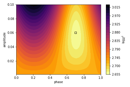
It looks like \(\chi^2\) is minimized near the input phase and amplitude (marked with a square)! But what about an actual measurement and uncertainty for these parameters? For this we use the likelihood function to convert these to relative probabilities, where \(L\propto\exp{-\chi^2/2}\) for Gaussian distributed noise. These are not properly normalized, so we just force the probabilities to sum to unity. Then we marginalize (sum) over each parameter to obtain a probability density estimate for the other.

# Convert these chi squared values to likelihoods
likelihoods = np.exp(-0.5*chisq)

# Normalize 
likelihoods /= np.sum(likelihoods)

# Marginalize over each parameter for the pdf of the other
amplikelihoods = np.sum(likelihoods,axis=0)
phaselikelihoods = np.sum(likelihoods,axis=1)

We plot the results and report the inferred values with uncertainties. We obtain medians by integrating the distributions to a value of 0.5, and the standard deviation is estimated as half the width of the region containing an inner 68.27% of the probability.

fig,axs = plt.subplots(1,2, figsize=(6,3))

# Plot pdf of sinusoidal phase over the grid
axs[0].bar(phasesample,phaselikelihoods,width=np.diff(phasesample)[0],color='0.7')

# Report the median and empirical standard deviation for the phase
percentile = interp1d(np.cumsum(phaselikelihoods),phasesample)
phasemed = percentile(0.5)
phaseerr = (percentile(1.-0.15865) - percentile(0.15865))/2.
axs[0].errorbar(phasemed,np.max(phaselikelihoods)*.5,xerr=phaseerr, c='k', 
                lw=2, capsize = 4, capthick = 2, label = 'measured')

# Compare to the underlying phase value and the analytically expected 
# uncertainty from a least squares fit
expectedphaseerr = np.sqrt(2./len(tsample))*noise/(amp*2.*np.pi)
axs[0].errorbar(phase,np.max(phaselikelihoods)*.55,xerr=expectedphaseerr, c='red', 
                lw=2, capsize = 4, capthick = 2, label = 'expected')

axs[0].set_ylabel('prob. density')
axs[0].set_xlabel('phase')
axs[0].set_xlim(np.min(phasesample),np.max(phasesample))
axs[0].legend()

# Plot pdf of sinusoidal amplitude over the grid
axs[1].bar(ampsample,amplikelihoods,width=np.diff(ampsample)[0],color='0.7')

# Report the median and empirical standard deviation for the amplitude
percentile = interp1d(np.cumsum(amplikelihoods),ampsample)
ampmed = percentile(0.5)
amperr = (percentile(1.-0.15865) - percentile(0.15865))/2.
axs[1].errorbar(ampmed,np.max(amplikelihoods)*.5,xerr=amperr, c='k', 
                lw=2, capsize = 4, capthick = 2, label = 'measured')

# Compare to the underlying phase value and the analytically expected 
# uncertainty from a least squares fit
expectedamperr = np.sqrt(2./len(tsample))*noise
axs[1].errorbar(amp,np.max(amplikelihoods)*.55,xerr=expectedamperr, c='red', 
                lw=2, capsize = 4, capthick = 2, label = 'expected')

axs[1].set_ylabel('prob. density')
axs[1].set_xlabel('amplitude')
axs[1].set_xlim(np.min(ampsample),np.max(ampsample))

plt.tight_layout()
plt.show()

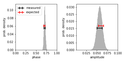
Yay! We have parameter estimates and the empirical uncertainties from the marginalized probability density functions match the precision expected from least-squares fitting (derived analytically by Montgomery & O’Donoghue 1999, Delta Scuti Star Newsletter, vol. 13, p. 28), as they should.

Needless to say I will never grid fit sinusoidal parameters like this again, but I managed to convince my colleague and we are moving forward with the statistical treatment that I suggested.