Inclination angles and a uniform distribution for isotropy
Here’s a little math problem that I’ve done enough times to warrant writing down somewhere: how can we most efficiently represent and randomly draw isotropic inclination angles? (spoiler: they’re uniform in \(\cos{i}\).)
A useful quantity to know in many astronomical situations is the inclination angle of some system. In my work, this is usually the orientation angle of a stellar rotation axis or the orbital plane of a binary star system. This is the angle with respect to the line of sight of the observer as depicted in this diagram:
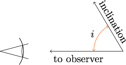
To help remember how the inclination angle, \(i\), is defined, I use the mnemonic that an elliptical orbit with zero inclination looks like a zero. The angle is defined for \(0^\circ < i < 90^\circ\) (\(0 < i < \pi/2\) radians), since we are only interested in the projected magnitude along our line of sight.
Our measurements are often only sensitive to the projections of quantities onto our line of sight or onto the “plane” of the sky. Since the projection does not equal the full magnitude of the quantity under investigation, this leads to so-called \(\sin{i}\) ambiguities. Such ambiguous measurements can be interpreted as lower/upper limits on physical values, interpreted statistically in the context of many objects, or used in conjunction with other measurements to empirically constrain \(i\).
Without good reason to think otherwise, we should expect a random object to be oriented randomly. Our knowledge of its inclination angle can be represented by an “isotropic” probability density function (p.d.f.), meaning all orientations are equally likely. The figure below will help us to write this down so that it is mathematically useful.
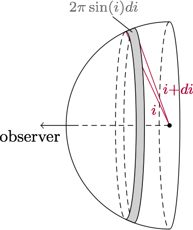
I’ve only drawn the observer-side hemisphere because the other half is merely a reflection. If a vector is equally likely to be oriented toward any part of the sphere, the relative likelihood that it falls within some small range \(di\) of a specific inclination angle is proportional to the area on the unit sphere covered by that range of angles. According to the figure above, the solid angle subtended by the inclination range \(i\) to \(i+di\) equals \(2\pi\sin{i}\,di\). We can write down the p.d.f. of isotropic inclination angles as
\[f(i) =
\begin{cases}
0, & i < 0; \\\
\sin{i}, & 0 \le i \le \pi/2; \\\
0, & i > \pi/2,
\end{cases}\]
which we have normalized so that \(\int_{-\infty}^{\infty}f(i)di = 1\).
This is a very useful result! We now know how much more likely it is to observe systems with high inclination angles than those pointed toward us. With a p.d.f. in hand, we can now generate random inclination angles for Monte Carlo analyses. However, a sine-distribution is not the most convenient choice to generate random numbers from. An inefficient way to do this would be to generate random numbers between 0 and \(\pi/2\), rejecting many in proportion to \(1-\sin{i}\) where the p.d.f. says inclinations are less likely. If we could find a way to change variables to an inclination representation that has a flat distribution, we wouldn’t have to waste any randomly generated numbers.
Let’s call the variable that we seek \(y\), and let it relate to \(i\) through a function \(i(y)\). Some narrow range \(dy\) must contain the same fraction of isotropic orientations as the corresponding \(di\). While the p.d.f. of \(i\) is given by \(f(i)\) above, we seek a flat \(g(y)\) that relates to \(f(i)\) through1
\[f(i)di = f(i(y))\bigl\vert\frac{di}{dy}\bigr\vert dy = g(y)dy. \]
If we wish for \(g(y)\) to be constant (flat) over the relevant range, we can rearrange to get:
\[\bigl\vert\frac{di}{dy}\bigr\vert\propto 1/f(i(y)).\]
This relationship is satisfied by the transformation \(y=\cos{i}\), or \(i(y)=\arccos{y}\), since \(1/f(i(y)) = \bigl\vert\frac{di}{dy}\bigr\vert = 1/\sqrt{1-y^2}\).
So we finally arrive at our very useful result that \(\cos(i)\) is uniformly distributed for isotropic inclination angles, yielding the easy-to-draw-from p.d.f.:
\[g(\cos{i}) =
\begin{cases}
0, & \cos{i} < 0; \\\
1, & 0 \le \cos{i} \le 1; \\\
0, & \cos{i} > 1.
\end{cases}\]
1: This method of changing variables of a p.d.f. is covered in Section 1.2.3. of E. L. Robinson’s excellent book Data Analysis for Scientists and Engineers. E.L.R. also taught me the mnemonic for remembering which orientation corresponds to \(i=0\), among many other things.
Astronomy, statistics, programming in Python, data visualization, data science, and other great icebreakers.
- Bootstrapping a significance threshold for periodogram analysis
- How data sampling affects the Fourier transform periodogram
- Three statistical tests for average spacing among numbers
- Confidence intervals for 2D Gaussian mixture models with contours
- What's the expected average value of a noisy amplitude spectrum?