In time domain research, it is well understood that the pattern of observations in time manifests itself in the frequency domain as a set of aliases that can confuse your identification of intrinsic frequencies. Conversely, if you want to avoid confusion in your frequency measurements, you should time your observations strategically.

Telescope time is expensive and competitive, so the observer has a responsibility to use that time efficiently. Sometimes more observations are not better than smart observations. I want to review an important paper that helped me learn how to observe smarter and to explain how to apply the insights to problems from my own work. The paper, “Variable stars: Which Nyquist frequency?” by L. Eyer and P. Bartholdi (1999, A&AS, 135, 1), is one of my favorites at only 3 pages long, and I think it should be required reading for every time-domain astronomer. It makes two main points:

1. The Nyquist frequency (see my previous post Nyquist analysis and the pyquist module) for irregularly sampled data is \(1/(2p)\), where \(p\) is the greatest common divisor of all of spacings in time between all pairs of observations. This is often very much higher than incorrect values commonly quoted in the literature that replace \(p\) with either the average or smallest time between observations.
2. The height of an alias in the observational spectral window (the characteristic signature about a coherent signal in the Fourier domain) is equal to the offset of the center of gravity of the observation times phase-folded on the alias frequency.

In this post, I focus on this second point and explore how this can be exploited to obtain better data. First, I will demonstrate the argument that I put forward in a white paper (Bell et al. 2018, arXiv:1812.03142) for this effect to be considered while executing the sparse time-domain observations of the Large Synoptic Survey Telescope (LSST). Then I will provide another simple example from my work on how the strategy for observing an individual target can be improved by considering the connection between observation timing and frequency aliases.

LSST will observe every part of the southern sky several hundred times over a ten year survey. They put out a call for white papers to weigh in on how these observations should be collected (the survey cadence), and they have also developed a sophisticated simulation framework for studying the effect of this cadence on the science that can be done with the data.

The figure below shows the spectral window (the Fourier transform of a constant value sampled as the observations) of a field in a simulated realization of the main LSST survey after three years. Peaks in the spectral window are called aliases and they can cause intrinsic signal frequencies to be misidentified as being offset by the alias frequency, especially in noisy data. The highest peak in this example at 11.6 micro-Hertz is the diurnal alias that is practically unavoidable in single-site observations that are limited to night-time. Basically, because you can’t observe during the day, there’s some ambiguity about exactly how many cycles of a periodic variation you missed when you weren’t observing, so multiple candidate frequencies can explain the (noisy) data pretty well. However, the other aliases present in this spectral window are easier to avoid and result from some other strict regularity in the observations.

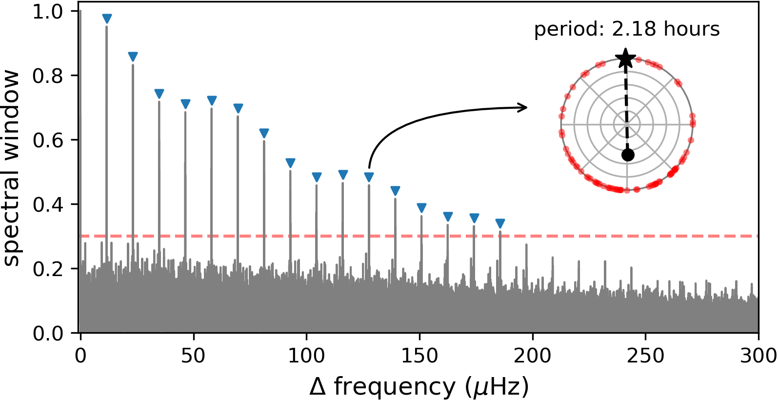
The polar plot inset in this figure demonstrates Eyer and Bartholdi’s point about alias peak heights equaling the center of gravity of the phase-folded time sampling. Here I’ve wrapped the observation times around a circle, folded on one alias period of 2.18 hours. The relative concentration of these points near the bottom of the circle cause the center of gravity to be offset by nearly half the radius, which is equal to the height of this alias peak. This applies for every frequency of the spectral window.

The actionable takeaway is that future observations can be timed to move these centers of gravity toward the middle of the circle, reducing the alias amplitudes. In the next figure, I show how the timing of a single new observation will change each of the marked alias amplitudes from the previous figure. Green means the amplitude is reduced, and red means the alias grows in amplitude. The bottom panel shows the effect on the combined heights of the set of marked aliases.

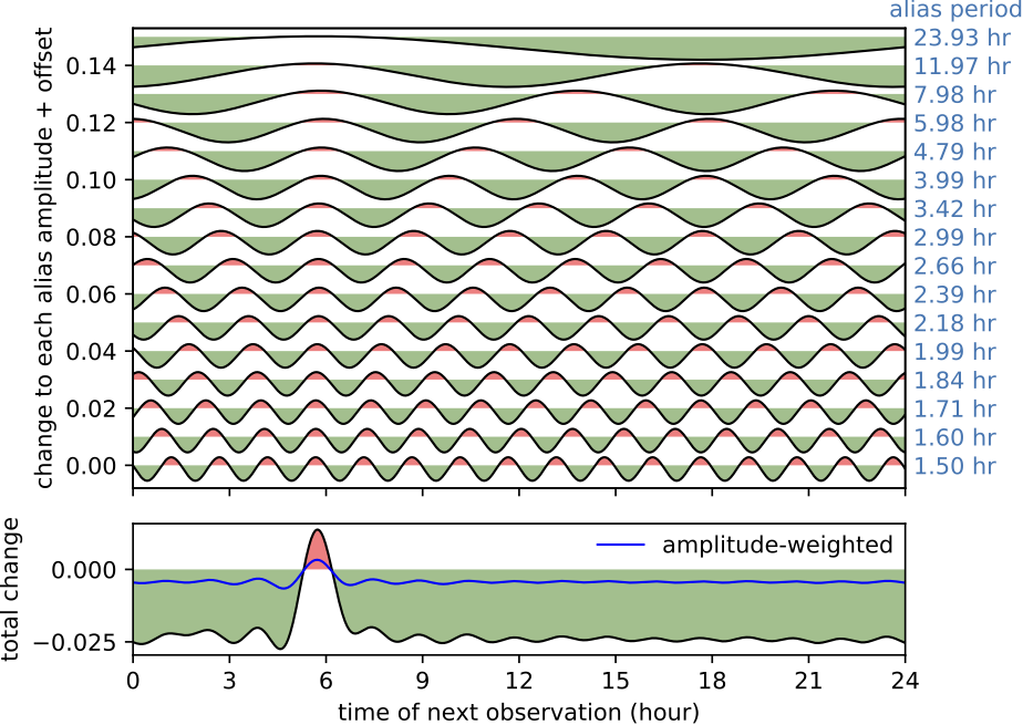
We see that the situation is improved as long as the next observation does not reinforce the strong concentration of observations near hour 6. Aliasing can be made less of a problem for the time-domain LSST data if this effect is taken into consideration as the timing of the survey observations is decided.

For one more example of how this concept can be applied in practice, let’s consider an interesting cataclysmic variable binary system SDSS J135154.46-064309.0. We (Green et al. 2018, MNRAS, 477, 5646) discovered this variable system in space-based time series photometry from the K2 mission. These data revealed two signals with periods near 16 minutes, separated by precisely 25.08 micro-Hertz. This is close to two times the typical diurnal frequency. We expect that one of these signals corresponds to the orbital frequency of the binary system that will also produce a signature of line shifts in time series spectroscopy. Determining which of these two photometric signals has a corresponding spectroscopic signal is important for characterizing this system.

Unfortunately we did not fully appreciate the problem we were trying to solve when we designed our first experiment to make this spectroscopic measurement. We did measure a large radial velocity signature, but the timing of our observations prevented us from being able to identify which photometric frequency was associated with the spectroscopic signal.

We have since devised a better strategy for obtaining these spectroscopic observations. Since we know that the two candidate signals are separated by precisely 25.08 micro-Hertz, we want to observe at times that avoid an alias at this frequency. Because this is not an exact multiple of the diurnal alias frequency, there will be a slight difference in phase between the two candidate frequencies on different nights. Measuring this phase tests the competing hypotheses of which photometric frequency the spectroscopic signal is associated with.

We use the center-of-gravity approach to compute the alias amplitude at 25.08 micro-Hertz that results from measuring the 16-minute spectroscopic variations on different combinations of nights.

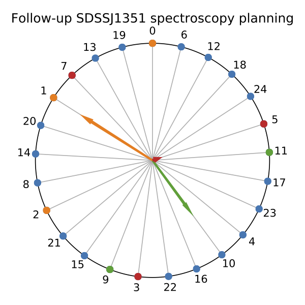
The orange arrow in the figure above shows the alias amplitude produced by observing on three consecutive nights (nights 0, 1, and 2). This is basically what we did in the original paper, and the measurements were too noisy to pick out the intrinsic frequency from the resulting set of alias peaks. If one of those nights is lost to weather, the situation could even be worse.

The red arrow shows the small alias amplitude produced if the three nights of observations are instead obtained every other night (nights 3, 5, and 7). This should make the photometric orbital signature very easy to identify. Even if one of these nights is lost, the alias amplitude represented by the green arrow is still lower than obtained from consecutive observing nights.

We have applied to obtain new observations of this system with this new strategy. Fingers crossed!

These have only been two examples of how understanding the connection between aliasing and observation timing can inform sound observing strategies. This concept can also helpful for analyzing data that are already in hand.

I love a good puzzle, so feel free to reach out via email or Twitter if you have any other problems of this sort that you’d like to discuss.